This paper is available on arxiv under CC 4.0 license.
Authors:
(1) Edson Pindza, Tshwane University of Technology; Department of Mathematics and Statistics; 175 Nelson Mandela Drive OR Private Bag X680 and Pretoria 0001; South Africa [[email protected]];
(2) Jules Clement Mba, University of Johannesburg; School of Economics, College of Business and Economics and P. O. Box 524, Auckland Park 2006; South Africa [[email protected]];
(3) Sutene Mwambi, University of Johannesburg; School of Economics, College of Business and Economics and P. O. Box 524, Auckland Park 2006; South Africa [[email protected]];
(4) Nneka Umeorah, Cardiff University; School of Mathematics; Cardiff CF24 4AG; United Kingdom [[email protected]].
Table of Links
- Abstract and Introduction
- Methodology
- Neural Network Methodology
- Numerical results, implementation and discussion
- Conclusion, Acknowledgments, and Funding
- Availability of data, code and materials, Contributions and Declarations
- References
3. Neural Network Methodology
The neural network (NN) algorithm is used for solving problems relating to dimensionality reduction [42, 49], visualization of data [31], clustering [11, 52] and classification issues [37, 40]. It is also used in regression [2, 21, 45] in solving regression problems since they do not require prior knowledge about the distribution of the data. The NN algorithm often has the tendency to predict with higher accuracy than other techniques due to the NN’s capability to fit any continuous functions [18]. Mathematically, the NN can be referred to as a directed graph having neurons as vertices and links as edges. Different forms of NN depend on the connectivity of their neurons, and the simplest one is the Multi-layer perceptron, also known as the feedforward NN. Basically, a NN can have only one input and one output layer in its simplest form, and this can be written as:

where m is the number of input variables, Φ is the activation function, wi,k is the weight of the input layer i with respect to the output k, b is the bias, and the input vector x is connected to the output k (denoting the kth neuron in the output layer) through a biased weighted sum. In the presence of hidden layers positioned between the input layers and the output layers, the output can be written as:

where m1 is the number of input variables, m2 is the number of nodes in the hidden layer, Φ : R → R refers to non-linear activation functions for each of the layers in the brackets, and Φout is the possibly new output function.
Recently, the NN has become an indispensable tool for learning the solutions of differential equations, and this section will utilize the potential of the NN in solving PDE-related problems [1, 10, 20, 50]. Also, the NN has been implemented in solving equations without analytical solutions. For instance, Nwankwo et al. [38] considered the solution of the American options PDE by incorporating the Landau transformation and solving the corresponding transformed function via a neural network approach. In many scientific and industrial contexts, there is a need to solve parametric PDEs using NN techniques and Khoo et al. [24] developed such a technique which solves PDE with inhomogeneous coefficient fields. For high-dimensional parametric PDE, [14] analyzed the deep parametric PDE method to solve high-dimensional parametric PDEs with much emphasis on financial applications.
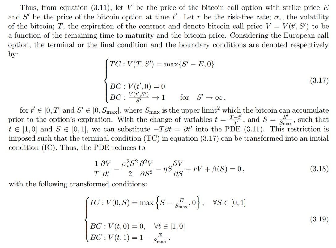
In the following, we describe the Bitcoin options with the corresponding Black-Scholes pricing PDE:

The above equation which is a non-homogeneous PDE can be re-written as
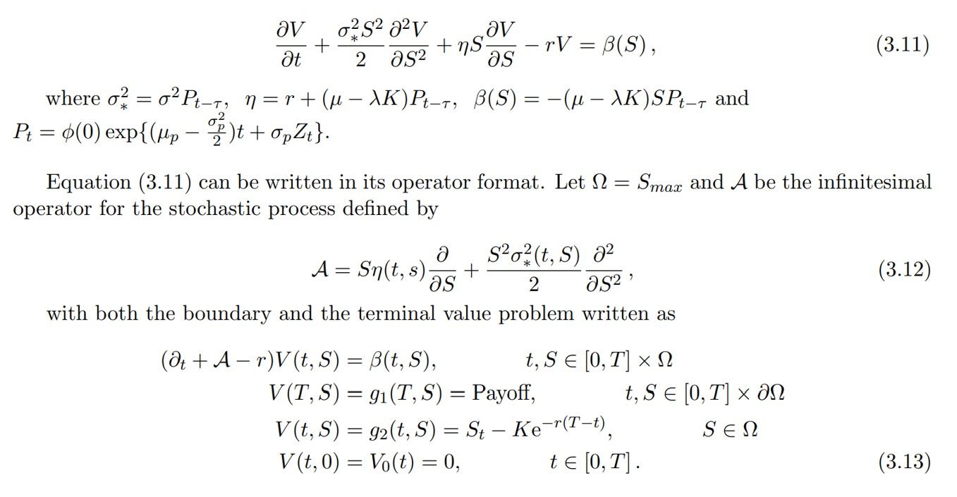
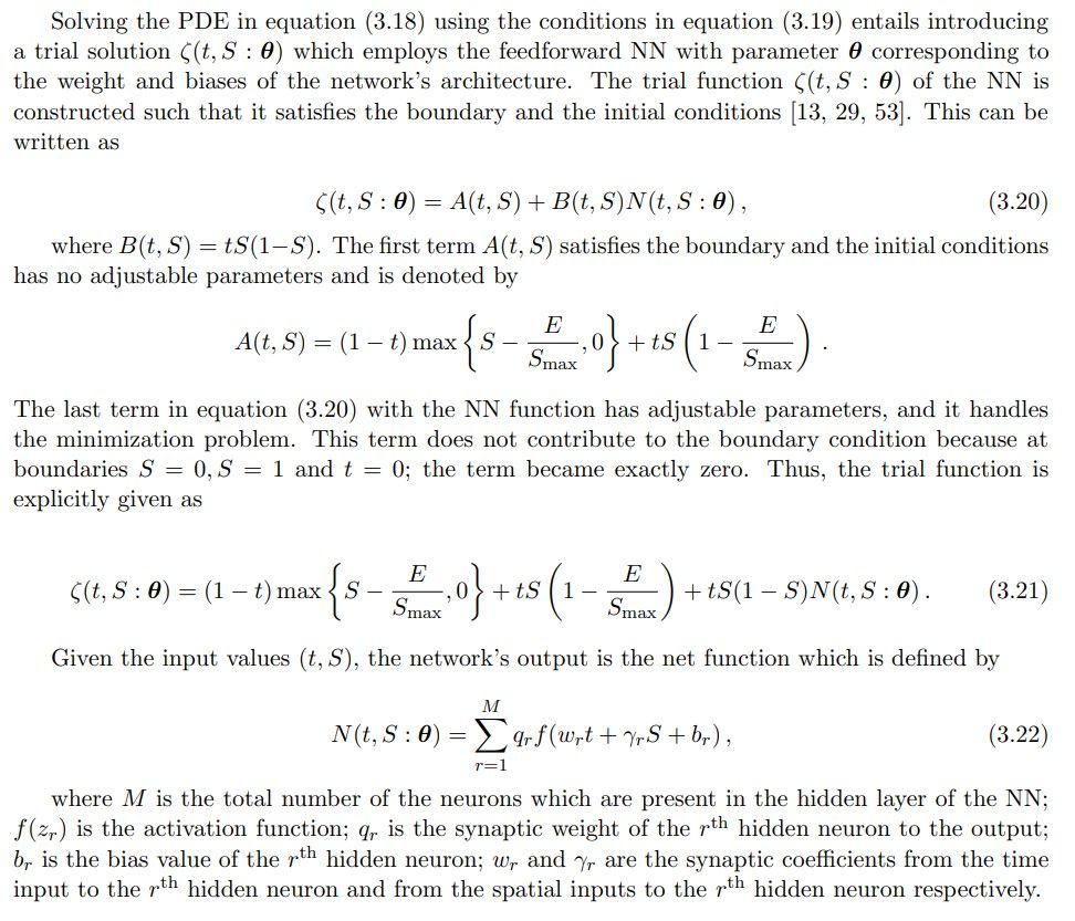
Standard theorems guarantee a classical smooth solution exists for the pricing PDE (3.13) given the assumed dynamics. The continuity and linear growth conditions on the coefficient functions ensure they satisfy Lipschitz continuity. Contingent claims theory shows that Lipschitz continuity is sufficient for existence and uniqueness under the stochastic process specifications. In particular, the smooth past price dependence in the diffusion coefficient allows the application results for delayed Black-Scholes equations. Therefore, the Cauchy problem is well-posed under the model assumptions, and a smooth pricing solution is guaranteed to exist based on the theorems. This provides the theoretical foundation for using a neural network to approximate the price function numerically. Thus, employing the ANN to solve the PDE, we introduce an approximating function ζ(t, S : θ) with parameter set θ. The loss or cost function associated with this training is measured by how well the approximation function satisfies the differential operator, boundary conditions and the terminal condition of the option pricing PDE. These are given respectively as
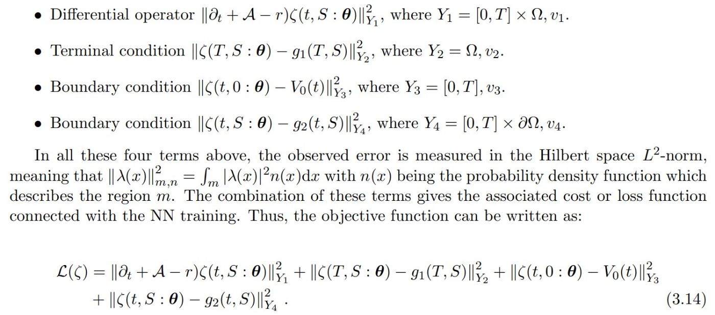
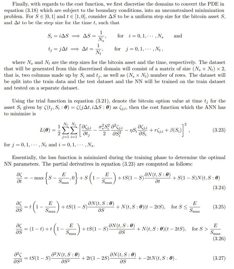
Suppose L(ζ) = 0, then ζ(t, S : θ) is a solution of the PDE in equation (3.13). The major aim is to obtain a set of parameters θ such that the function ζ(t, S : θ) minimizes the observed error of L(ζ). The procedure for seeking a good parameter set by minimizing this loss function using the stochastic gradient descent (SGD) optimizer is called “training”. Thus, using a Machine Learning approach, and in this case, the artificial NN, it will be feasible to minimize the function L(ζ) by applying the SGD approach on the sequence of asset and time points which are drawn at random. A part of the input samples, fully dependent on the mini-batch size, is drawn within each iteration to estimate the gradient of the given objective function. The gradient is then estimated over these mini-batches due to the limitations of the computer memory [30].
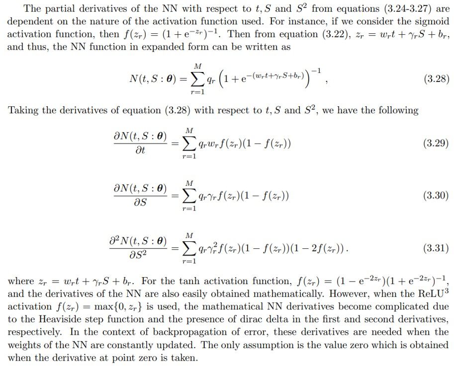
The training of NN is classified into first identifying the network’s hyperparameters, that is, the architectural structure and the loss function of the network. Next, use the SGD to optimize or estimate the loss minimizer, and then the derivatives of the loss function are computed using the backpropagation techniques. Essentially, the process of searching and identifying the best θ parameter by minimizing the loss function using the gradient descent-based optimizers is referred to as “training”. The whole procedure is well illustrated in the algorithm below [46], and can be implemented in solving the PDE in equation (3.13):
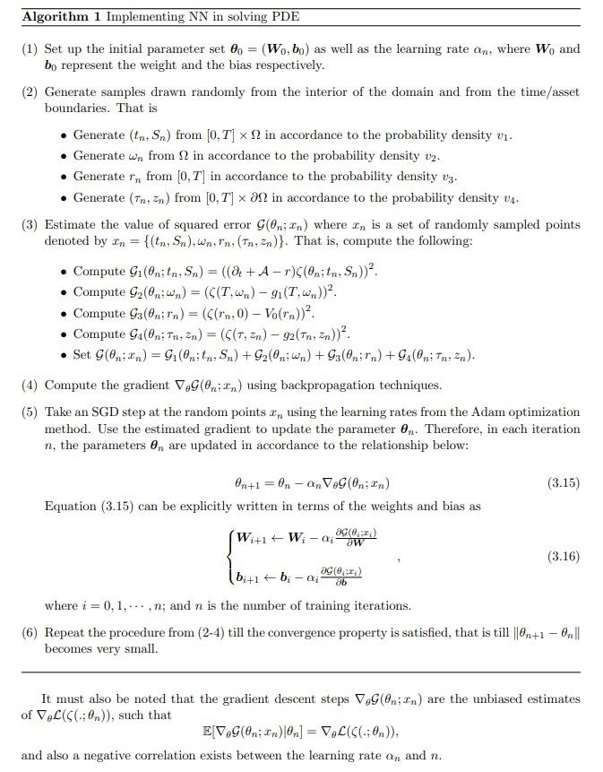
The learning rate α is employed to scale the intensity of the parameter updates during the gradient descent. Choosing the learning rate, as the descent parameter α, in the network training is crucial since this factor plays a significant role in aiding the algorithm’s convergence to the true solution in the gradient descent. It equally affects the pace at which the algorithm learns and whether or not the cost function is minimized. When α implies divergence, and thus, the optimal point can be missed. Also, a fixed value of α can most likely make the local optima overshoot after some iterations, leading to divergence. Defining the learning rate as a dynamic decreasing function is preferable since it allows the algorithm to identify the needed point rapidly. Another limitation in employing the gradient descent method is obtaining the value of the initial parameters of the loss function. If the value is significantly close to the local optimum, then the slope of the loss function reduces, thereby leading to the optimal convergence. Otherwise, there will be no convergence as the solution explodes abnormally.
3.1. Solution of bitcoin option pricing PDE
While the pricing PDE has a proven smooth solution under the model dynamics, obtaining the analytical form is intractable. Numerical methods must be used to approximate the solution. Neural networks provide a flexible parametric approach based on their universal approximation theoretical results. Given sufficient network capacity, neural networks can represent a wide class of functions, including solutions to PDEs like the pricing equation. However, challenges remain in finding the optimal network parameters to recover the true solution robustly. While existence is guaranteed, the non-convex optimization of neural networks does not assure convergence to global optimality. Care must be taken in specifying the network architecture, loss function, regularization, and training methodology to promote the learning of the pricing function. Subject to these caveats, neural networks present a promising computational technique for approximating smooth pricing solutions, circumventing discretization of the domain. We note the limitations of using neural networks as function approximators. However, their generalization capabilities provide a methodology for data-driven extraction of the pricing mapping across the entire domain. This avoids the constraints of methods like grid-based techniques that rely on local consistency. Future work should explore neural network training enhancements and theoretical guarantees to ensure robust solutions.
